Parallel Coordinates

Hint

Conveys a dense overview of the trial objectives in a multi-dimensional space. Helps identifying trends of best or worst hyperparameter values.

The parallel coordinates plot decomposes a search space of n dimensions into n axis so that the entire space can be visualized simultaneously. Each dimension is represented as a vertical axis and trials are represented as lines crossing each axis at the corresponding value of the hyperparameters. There is no obvious optimal ordering for the vertical axis, and you will often find that changing the order helps better understanding the data. Additionally, the lines are plotted with graded colors based on the objective. The gradation is shown in a color bar on the right of the plot. Note that the objectives are added as the last axis is the plot as well.

orion.plotting.base.parallel_coordinates(experiment, with_evc_tree=True, order=None, **kwargs)

Make a Parallel Coordinates Plot to visualize the effect of the hyperparameters on the objective.

Parameters

experiment: ExperimentClient or Experiment

The orion object containing the experiment data

with_evc_tree: bool, optional

Fetch all trials from the EVC tree. Default: True

order: list of str or None

Indicates the order of columns in the parallel coordinate plot. By default the columns are sorted alphabetically with the exception of the first column which is reserved for a fidelity dimension is there is one in the search space.

kwargs: dict

All other plotting keyword arguments to be passed to plotly express.line.

Returns

plotly.graph_objects.Figure

Raises

ValueError

If no experiment is provided.

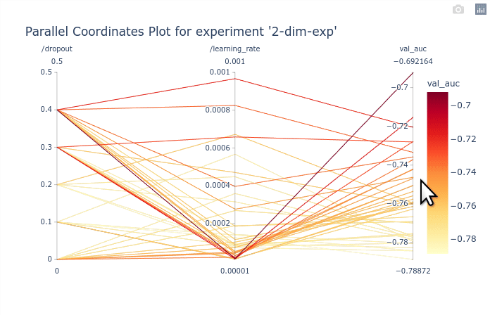
The parallel coordinates plot can be executed directly from the experiment with plot.parallel_coordinates() as shown in the example below.

from orion.client import get_experiment

# flake8: noqa

# Specify the database where the experiments are stored. We use a local PickleDB here.
storage = dict(type="legacy", database=dict(type="pickleddb", host="../db.pkl"))

# Load the data for the specified experiment
experiment = get_experiment("2-dim-exp", storage=storage)
fig = experiment.plot.parallel_coordinates()
fig

algorithms is deprecated and will be removed in v0.4.0. Use algorithm instead.
`strategy` option is not supported anymore. It should be set in algorithm configuration directly.

In this basic example the parallel coordinates plot is marginally useful as there are only 2 dimensions. It is possible however to identify the best performing values of dropout and learning_rate. The GIF below demonstrates how to select subsets of the axis to highlight the trials that corresponds to the best objectives.

Note

Hover is not supported by plotly at the moment. Feature request can be tracked here.

Lets now load the results from tutorial Checkpointing trials for an example with a larger search space.

# Load the data for the specified experiment
experiment = get_experiment("hyperband-cifar10", storage=storage)
fig = experiment.plot.parallel_coordinates()
fig

algorithms is deprecated and will be removed in v0.4.0. Use algorithm instead.
`strategy` option is not supported anymore. It should be set in algorithm configuration directly.

As you can see, the large number of trials until trained for a few epochs is cluttering the entire plot. You can first select the trials with 120 epochs to clear the plot. Once that is done, We can see that gamma and momentum had limited influence. Good trials can be found for almost any values of gamma and momentum. On the other hand, learning rate and weight decay are clearly more optimal in lower values. You can try re-ordering the columns as shown in the animation below to see the connections between one hyperparameter and the objective.

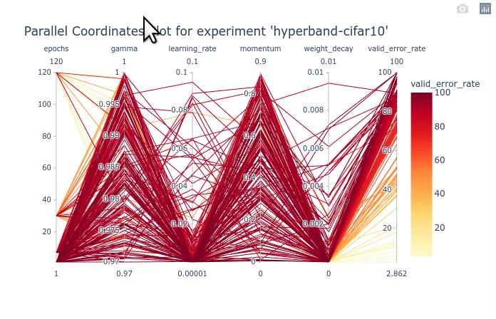
We can also select a subset of hyperparameters to help with the visualization.

# Load the data for the specified experiment
fig = experiment.plot.parallel_coordinates(
    order=["epochs", "learning_rate", "weight_decay"]
)
fig

Special cases

Logarithmic scale

Note

Logarithmic scales are not supported yet. Contributions are welcome. :) See issue.

Dimension with shape

If some dimensions have a shape larger than 1, they will be flattened so that each subdimension can be represented in the parallel coordinates plot.

# Load the data for the specified experiment
experiment = get_experiment("2-dim-shape-exp", storage=storage)
fig = experiment.plot.parallel_coordinates()
fig

algorithms is deprecated and will be removed in v0.4.0. Use algorithm instead.
`strategy` option is not supported anymore. It should be set in algorithm configuration directly.

In the example above, the dimension learning_rate~loguniform(1e-5, 1e-2, shape=3) is flattened and represented with learning_rate[i]. If the shape would be or more dimensions (ex: (3, 2)), the indices would be learning_rate[i,j] with i=0..2 and j=0..1.

The flattened hyperparameters can be fully selected with params=['<name>'].

experiment.plot.parallel_coordinates(order=["/learning_rate"])

Or a subset of the flattened hyperparameters can be selected with params=['<name>[index]'].

experiment.plot.parallel_coordinates(order=["/learning_rate[0]", "/learning_rate[1]"])

Categorical dimension

Parallel coordinates plots can also render categorical dimensions, in which case the categories are shown in an arbitrary order on the axis.

# Load the data for the specified experiment
experiment = get_experiment("3-dim-cat-shape-exp", storage=storage)
fig = experiment.plot.parallel_coordinates()
fig

algorithms is deprecated and will be removed in v0.4.0. Use algorithm instead.
`strategy` option is not supported anymore. It should be set in algorithm configuration directly.

Finally we save the image to serve as a thumbnail for this example. See the guide How to save for more information on image saving.

fig.write_image("../../docs/src/_static/pcp_thumbnail.png")